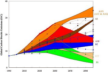
Figure 6-7: Global CO2 emissions
(GtC, standardized) from all sources for the four scenario families
from 1990 to 2100. Scenarios are also presented for the four constituent
groups of the A1 family (high-coal A1C, high oil and gas A1G, high non-fossil
fuel A1T, and the balanced A1B) and for the other three families (A2,
B1, and B2), forming seven scenario groups altogether. The emissions
of A1C and A1G scenario groups are combined into A1FI (see footnote
2). Each colored emission band shows the range of the harmonized
scenarios within one group that share common global input assumptions
for population and GDP. The scenarios remaining outside the seven groups
adopted alternative interpretations of the four scenario storylines.
|
6.3.1.2. Four Categories of Cumulative Emissions
This comparison of some of the SRES scenario characteristics implies that similar
future emissions can result from very different socio-economic developments,
and similar developments of driving forces can result in different future emissions.
Uncertainties in the future development of key emission driving forces create
large uncertainties in future emissions, even within the same socio-economic
development paths. Therefore, emissions from each scenario family overlap substantially
with emissions from other scenario families. Figure 6-6
shows this for CO2 emissions. For example, comparison of the A1B and B2 marker
scenarios indicates that they have similar emissions of about 13.5 and 13.7
GtC by 2100, respectively. The dynamics of the paths, however, are different
so that they have different cumulative CO2 emissions and different emissions
of other GHG gases and SO2 .
To facilitate comparisons of emissions and their driving forces across the
scenarios, the writing team grouped them into four categories of cumulative
emissions between 1990 and 2100. However, any categorization of scenarios based
on emissions of multiple gases is quite difficult. Figure
6-7 shows total CO2 emissions from all sources (from Figures
6-6a and b). Most of the scenarios are shown aggregated into seven groups,
the four A1 groups and the other three families. The scenarios that remain outside
the seven groups adopted alternative interpretations of the four scenario storylines.
The emission trajectories ("bands") of the seven groups display different dynamics,
from monotonic increases to non-linear trajectories in which there is a subsequent
decline from a maximum. The dynamics of the individual scenarios are also different
across gasses, sectors, or world regions. This particularly diminishes the significance
of focusing scenario categorization on any given year, such as 2100. In addition,
all gases that contribute to radiative forcing should be considered, but methods
of combining gases such as the use of global warming potentials (GWP) are appropriate
only for near-term GHG inventories4.
In light of these difficulties, the classification approach presented here uses
cumulative CO2 emissions between 1990 and 2100. CO2 is the dominant GHG and
cumulative CO2 emissions are expected to be roughly proportional to CO2 radiative
forcing over the time scale of a century. According to the IPCC SAR, "any eventual
stabilised concentration is governed more by the accumulated anthropogenic CO2
emissions from now until the time of stabilisation than by the way emissions
change over the period" (Houghton et al., 1996). Therefore, the writing
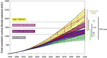
team also grouped the scenarios according to their cumulative emissions (see
Figure 6.8).

Figure 6-8: Global cumulative
CO2 emissions (GtC, standardized). The ranges of cumulative emissions
for the SRES scenarios are shown. Scenarios are grouped into four categories:
low, medium-low, medium-high, and high emissions. Each category contains
one marker scenario plus alternatives that lead to comparable cumulative
emissions, although often through different driving forces. The ranges
of cumulative emissions of the SRES scenario groups are shown as colored
vertical bars and the range of the IS92 scenarios as a black vertical
bar. (See also footnote
2).
|
This categorization can guide comparisons using either scenarios with different
driving forces yet similar emissions, or scenarios with similar driving forces
but different emissions. This characteristic of SRES scenarios also has very
important implications for the assessment of climate-change impacts, mitigation,
and adaptation strategies. Two future worlds with fundamentally different characteristic
features, such as the A1 and B2 marker scenarios, also have different cumulative
CO2 emissions, but very similar CO2 emissions in 2100. In contrast, scenarios
that are in the same category of cumulative emissions can have fundamentally
different driving forces and different CO2 emissions in 2100, but very similar
cumulative emissions. Presumably, adverse impacts and effective adaptation measures
would vary among the scenarios from different families that share similar cumulative
emissions, but have different demographic, socio-economic, and technological
driving forces. This is another reason for considering the entire range of emissions
in future assessments of climate change.
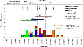
Figure 6-9 shows the histogram of cumulative CO2
emissions from 1990 to 2100 for the SRES scenarios subdivided into the four
emissions categories. Relative positions of the four marker scenarios, and the
ranges of the four families and the six IS92 scenarios, are marked. The SRES
scenarios have a bimodal structure similar to the distribution of cumulative
emissions from the scenarios in the literature. The groups of SRES scenarios
span the whole range of cumulative emissions from the scenarios in the literature.
The range of the four markers is from 1000 to 1900 GtC. In comparison, the IS92
cumulative emissions range from 700 GtC for IS92c to 2140 GtC for IS92e.
The SRES emissions scenarios encompass emissions of other GHGs and chemically
active species such as carbon monoxide, nitrogen oxides, and non-methane volatile
organic compounds. The emissions of other gases follow dynamic patterns much
like those shown in Figures 6-5 and 6-6
for CO2 emissions. Further details of GHG emissions are given in Chapter
5.

Figure 6-9: Global cumulative
CO2 emissions of the SRES scenarios. Relative positions of the marker
scenarios and the A1 scenario groups are shown on the histogram. The
40 SRES scenarios have median cumulative emissions of about 1500 GtC.
(See also footnote
2).
|
